
Stable distributions, also known as Lévy stable distributions, offer a powerful alternative to the normal distribution in financial modeling, particularly when dealing with asset returns. Their defining characteristic is *stability*, meaning that a linear combination of independent random variables drawn from a stable distribution also follows a stable distribution (with the same stability parameter). This property is crucial for modeling portfolio returns, as it ensures consistency across aggregation. Unlike the normal distribution, stable distributions can capture the “fat tails” and skewness often observed in financial data, reflecting the higher probability of extreme events (market crashes, unexpected booms) than predicted by a normal distribution.
The stability parameter, α (0 < α ≤ 2), dictates the tail heaviness. A lower α corresponds to heavier tails and a greater probability of extreme events. When α = 2, the stable distribution reduces to the normal distribution. The parameter β (-1 ≤ β ≤ 1) governs skewness, with β = 0 indicating symmetry, β > 0 indicating right skew (longer right tail), and β < 0 indicating left skew (longer left tail). Two additional parameters, scale (σ) and location (μ), determine the spread and center of the distribution, respectively, similar to the standard deviation and mean in a normal distribution.
The relevance to finance stems from the limitations of the normal distribution. Many financial assets exhibit non-normal return distributions. Extreme events, often driven by factors outside of standard risk models, occur more frequently than predicted by a normal curve. Using a normal distribution can thus underestimate risk, leading to inadequate risk management strategies. Stable distributions, with their ability to accommodate fat tails, offer a more realistic representation of these risks.
For example, in portfolio optimization, using stable distributions allows for constructing portfolios that are more robust to extreme market movements. Value at Risk (VaR) and Expected Shortfall (ES) calculations based on stable distributions provide a more accurate estimate of potential losses compared to calculations based on normality assumptions. Option pricing can also benefit; stable distributions can be incorporated into models to account for the higher volatility and extreme price jumps often observed in options markets.
However, stable distributions also present challenges. They generally lack closed-form expressions for their probability density function and cumulative distribution function, except in a few special cases (normal, Cauchy, and Lévy distributions). Parameter estimation can be computationally intensive and sensitive to data quality. Furthermore, the infinite variance of stable distributions when α < 2 raises theoretical concerns about traditional statistical measures based on variance. Despite these challenges, the ability of stable distributions to capture stylized facts of financial data makes them a valuable tool for risk management, portfolio optimization, and derivative pricing, particularly when dealing with assets exhibiting significant tail risk.
 1200×1200 stable finance from medium.com
  494×478 stable distribution function wolfram demonstrations project from demonstrations.wolfram.com
  1150×724 stable distribution wolfram mathworld from mathworld.wolfram.com
  560×420 stable distribution matlab simulink from www.mathworks.com
  1024×330 stable dividend policy definition implementation from corporatefinanceinstitute.com
  933×1764 stable money trusted platform bonds fixed deposits from stablemoney.in
  756×444 solved find stable distribution regular cheggcom from www.chegg.com
  884×497 stablecoins decentralized finance smart liquidity research from smartliquidity.info
  768×512 mastering data distribution stable diffusion tips from blog.daisie.com
  320×320 comparing fitted normal stable distribution scientific from www.researchgate.net
  500×351 stable distribution model stock prices mathematica from www.wolfram.com
 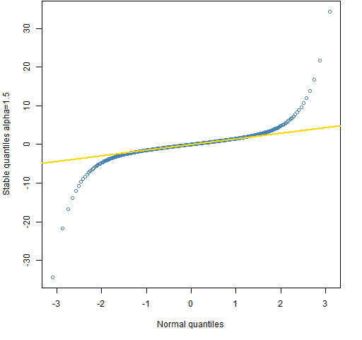 512×480 introduction stable distributions finance bloggers from www.r-bloggers.com
  744×1024 finding stable distribution regular from studylib.net
  512×512 stable diffusion distribution assets geek culture medium from medium.com
  1732×511 stable diffusion pricing features reviews apr from www.softwaresuggest.com
  3514×2683 introducing stable distributions blog from notepad.michaelpershan.com
  786×432 stablecoins navigating everyday finances stability from blog.digifortune.net
  621×397 stable distribution simulations scenarios alpha from www.researchgate.net
  1151×896 scam dont invest stable dividends review hyip investors from hyipinvestors.org
  800×800 financially stable dividend income investor from www.dividendincomeinvestor.com
  3242×1047 itim retail software solutions stock distribution from www.itim.com
  738×927 influence parameters shape stable distribution from www.researchgate.net
  1200×675 role stablecoins decentralized finance sevenhash medium from medium.com
  758×745 financially stable wealth diagram from wealthdiagram.com
  398×398 compare stable distributions scientific diagram from www.researchgate.net
  1024×614 hire stable diffusion developers stable diffusion development from rejolut.com
  1302×698 stablecoin liquidity diving data kaiko research from research.kaiko.com
  626×351 premium ai image stable fixed income investments from www.freepik.com
  850×1290 stable distributions from www.researchgate.net
  1200×627 hire stable diffusion developers enhance ai models from www.bacancytechnology.com
  626×351 premium ai image stable financial growth fixed income from www.freepik.com