
GARCH Models in Finance
Generalized Autoregressive Conditional Heteroskedasticity (GARCH) models are a cornerstone of financial time series analysis, specifically designed to capture the phenomenon of volatility clustering. Volatility clustering, the tendency for large changes in asset prices to be followed by more large changes, and small changes by more small changes, is a key characteristic of financial markets. Traditional time series models, like ARMA, often struggle to account for this non-constant variance over time. GARCH provides a framework for modeling and forecasting this changing volatility.
At its core, a GARCH model postulates that the conditional variance (volatility) of a time series depends on both past values of the series itself and past values of the variance. The most common form is the GARCH(p, q) model, where ‘p’ represents the order of the autoregressive (AR) component for the conditional variance, and ‘q’ represents the order of the moving average (MA) component for the squared residuals of the series.
The GARCH(1, 1) model is the most widely used specification due to its simplicity and ability to capture the essential features of volatility clustering. The equation for a GARCH(1,1) model can be represented as follows:
σt2 = ω + α εt-12 + β σt-12
Where:
- σt2 is the conditional variance at time t.
- ω is a constant representing the long-run average variance.
- α is the coefficient on the squared residual from the previous period (εt-12), representing the impact of past shocks on current volatility.
- β is the coefficient on the lagged conditional variance (σt-12), representing the persistence of volatility.
For the model to be stable, the parameters α and β must be non-negative, and their sum (α + β) should be less than 1. If (α + β) is close to 1, it indicates high volatility persistence; shocks to volatility take a long time to dissipate.
GARCH models have numerous applications in finance:
- Risk Management: Accurate volatility forecasts are crucial for value-at-risk (VaR) calculations and other risk management techniques.
- Option Pricing: Volatility is a key input in option pricing models like the Black-Scholes model. GARCH models can provide dynamic volatility estimates for more accurate pricing.
- Portfolio Optimization: Incorporating time-varying volatility into portfolio allocation strategies can lead to improved risk-adjusted returns.
- Volatility Trading: GARCH models can be used to identify periods of high or low volatility, which can inform trading strategies based on volatility expectations.
While GARCH models are powerful tools, they have limitations. They assume that positive and negative shocks have the same impact on volatility (symmetric response). Extensions like the EGARCH (Exponential GARCH) and GJR-GARCH models address this by allowing for asymmetric responses to shocks. Also, GARCH models can be sensitive to outliers and may require careful data cleaning. Despite these limitations, GARCH models remain indispensable for financial professionals needing to understand and manage volatility in financial markets.
 1024×682 garch model learnsignal from www.learnsignal.com
  389×255 github kinhrealized garch incorporating realized measure from github.com
  100×115 garch model finance from www.researchgate.net
  768×1087 garch model assignment from www.slideshare.net
768×1087 garch model assignment from www.slideshare.net 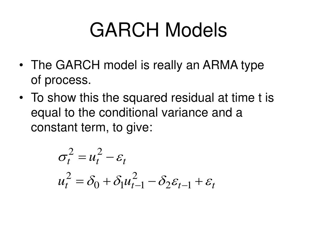 1024×768 garch models asymmetric garch models powerpoint from www.slideserve.com
  850×466 garch model specifications table from www.researchgate.net
  1536×1344 time series analysis generalized autoregressive conditional from vlyubchich.github.io
  556×514 garch model simple definition statistics from www.statisticshowto.com
  640×400 garch model aptech from www.aptech.com
  1024×768 module garch models powerpoint id from www.slideserve.com
  800×446 garch model ekonometri ders notlari from www.ekolar.com
  640×640 summary results garch type models table from www.researchgate.net
  850×237 garch model remittances exchange rate scientific diagram from www.researchgate.net
 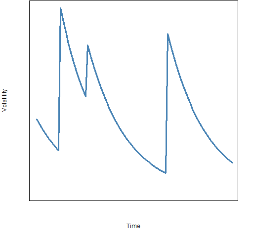 512×480 practical introduction garch modeling bloggers from www.r-bloggers.com
  850×97 selection garch model model scientific diagram from www.researchgate.net
  640×640 types garch models scientific diagram from www.researchgate.net
  850×831 arch garch model select banking companies scientific from www.researchgate.net
  1260×704 github davidalexandermoefinancial time series analysis from github.com
  320×320 garch model comprehensive modeling flow chart analysis from www.researchgate.net
  1039×812 finance garch model economics stack from economics.stackexchange.com
  640×640 volatility financial flows optimal garch model from www.researchgate.net
  850×564 variables included garch model scientific diagram from www.researchgate.net
  850×737 result garch models model selection scientific diagram from www.researchgate.net
  850×1202 performance realized garch model garch types from www.researchgate.net
  524×524 garch models leverage effect differences similarities from www.researchgate.net
  850×638 var garch models stock housing markets scientific from www.researchgate.net